Recursive Embedding Fine-Tuning: Learning Without Forgetting (the Funes Paradox in Production)

Q: What is recursive embedding fine-tuning?

It is the periodic, automated retraining of the model that turns text into vectors, on a corpus's new data, with a strict rule: a new version is promoted to production only if it beats the old one on a held-out test set. Each cycle chains LoRA training, golden evaluation, generalist-forgetting check, then cutover or rollback.

Q: What is the difference between Recall@k, MRR, and nDCG?

Recall@k measures whether the right document is returned in the top k results (coverage). MRR rewards ranking it high (1/rank of the first correct result). nDCG refines further by logarithmically penalizing correct answers placed low and accounting for graded relevance. For a RAG, MRR is the most important because the LLM mostly reads the first passages.

Q: What is catastrophic forgetting in fine-tuning?

It is the loss of a model's generalist skills when you specialize it too much on a singular corpus — the Funes paradox applied to the model. It is measured by evaluating the fine-tuned model on a generalist slice never seen during training; if its score drops beyond a threshold, promotion is refused.

Q: How do you guard against catastrophic forgetting?

Three cumulable techniques: rehearsal/replay (re-injecting samples from the original generalist corpus during training), a permanent held-out generalist evaluation as a safeguard, and a pre-training checkpoint with automatic rollback if the evaluation regresses. Keeping the backbone frozen via LoRA is a further protection by construction.

Q: Why is a gain measured on 40 questions not reliable?

Because the variance of a small sample dominates the signal. In a real case, an MRR gap of -0.027 on 40 questions fell to -0.016 as soon as it moved to 80 questions. Effect size must always be read alongside sample size: a gap on too few cases is not proof.

Q: Does fine-tuning always improve the model?

No. On a too-small dataset (50 pairs), the fine-tune degraded Recall@1 by -0.045. Adding off-distribution data lowered the MRR and triggered a rollback. More data or more training are only worth it if evaluated — that is the point of the empirical gate.

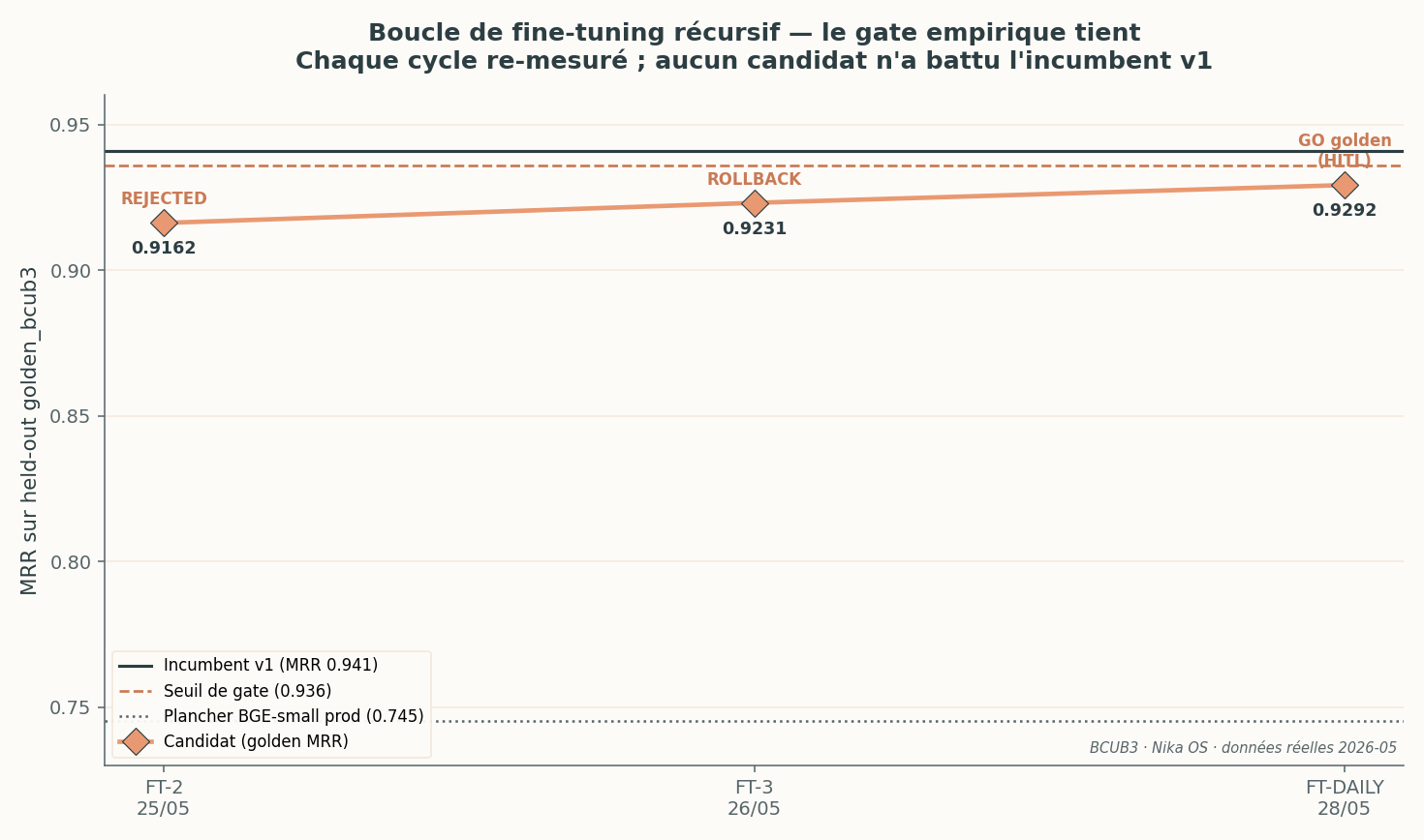Recursive embedding fine-tuning loop: the candidate's MRR re-measured at each cycle, compared to the production incumbent and the gate threshold. Three recursive fine-tuning cycles. No candidate crossed the v1 incumbent threshold — the empirical gate refused every promotion. That is the system working, not failing.

TL;DR

Recursive fine-tuning means continuously retraining the model that turns your text into vectors (the embeddings), measuring the real gain on a test set, and promoting a new version only if it beats the old one — with the numbers to prove it. On Nika OS, every cycle follows the same discipline: LoRA training on e5-base, evaluation on a held-out golden set, a generalist-forgetting check, then cutover or rollback.

The real numbers measured: moving from BGE-small (production) to fine-tuned e5-base yields +0.184 MRR and +15 points of Recall@10 on the BCUB3 golden set (n=100). But across three successive cycles, no candidate beat the v1 incumbent (MRR 0.9408) — the system refused them all. And the hunt for catastrophic forgetting — the Funes paradox applied to the model — showed that a too-small test slice (n=40) triggers a false alarm that vanishes the moment you double the sample (n=80). The core lesson: measure before you adopt; a model that “feels better” without a number has no right to ship.

What is recursive embedding fine-tuning?

The embedding, the base brick of RAG

An agent like Nika does not “read” your documents on every question. It has previously turned them into embeddings: numerical vectors (here 384 or 768 dimensions) that encode the meaning of a passage. When you ask a question, it too is turned into a vector, and the system returns the passages whose vector is closest. This is the heart of RAG (Retrieval-Augmented Generation): you retrieve before you answer, to anchor the answer in facts rather than in the model’s imagination.

The quality of the whole edifice therefore depends on one thing: does the embedding model place the right documents near the right questions? A generic model (trained on the web) knows the world but knows nothing of your internal vocabulary — your clients, your processes, your in-house acronyms. Hence the idea of specializing it.

Why retrain in a loop

The corpus of a living organization is not frozen: every day new emails, quotes, reports, and work sessions are added. A model fine-tuned once in May will be slightly off by July. Recursive fine-tuning addresses this drift: at a regular interval (here, a daily FT-DAILY cycle), you retrain on fresh data, re-measure, and decide.

The important phrase is you decide. A loop that retrains and promotes automatically, without a gate, is not learning: it is drifting. Recursion only has value because it is bounded by a measurement that can say no.

LoRA: specialize without breaking everything

We do not retrain the base model’s 110 million parameters at every cycle — that would be expensive and dangerous. We use LoRA (Low-Rank Adaptation): the original model is frozen, and we train only small low-rank matrices grafted on top. The real configuration of the Nika cycles:

Parameter	Value
Base model	`intfloat/multilingual-e5-base` (frozen)
LoRA rank / alpha / dropout	16 / 32 / 0.1
Learning rate	2 × 10⁻⁵
Epochs	3
Batch size	32
Warmup steps	100
Weight decay	0.01
Temperature (contrastive)	0.02
Seed	42 (deterministic)
Training pairs	11,058
Hardware	NVIDIA A100 80 GB
Duration	716 s (~12 min)
Cost	~$0.31/cycle

The fact that the backbone stays frozen is the first protection against catastrophic forgetting: the drift of the weights is bounded by construction. We return to this below.

Reading the indicators without being a data scientist

Before the curves, let’s set the vocabulary. These four indicators appear everywhere in the article.

Recall@k — “did I retrieve the right info?”

Recall@k is the proportion of questions for which the right document appears in the top k results. Recall@1 = the right document is in first position. Recall@10 = it is somewhere in the top ten. It is a coverage measure: regardless of the exact position, is the info there?

MRR — “is it ranked HIGH?”

MRR (Mean Reciprocal Rank) refines Recall by rewarding position. For each question, take 1 / rank of the first correct result, then average. Right document in position 1 → 1.0; in position 2 → 0.5; in position 4 → 0.25. A retriever that returns the right answer but in 8th position has good Recall@10 and poor MRR. For a RAG, MRR is the king indicator, because the LLM mostly reads the first passages.

nDCG — “is the ranking clean?”

nDCG (Normalized Discounted Cumulative Gain) goes further still: it logarithmically penalizes every correct answer placed low in the list and normalizes everything between 0 and 1. It accounts for position and graded relevance. It is the finest of the three.

Effect size vs p-value — “is the gain real or noise?”

Two distinct questions, often confused:

The p-value answers “is this result due to chance?”. A low p-value says “probably not chance.”
The effect size answers “is it big?”. A gain can be statistically detectable yet tiny, hence of no practical interest.

A p-value without effect size is noise, and an effect size on a tiny sample is fragile. You will see below a real case where a gap of −0.027 on 40 questions triggers an alarm that evaporates the moment you move to 80 questions: the sample size, not just the sign of the gap, decides.

The generalist-forgetting metric — “did I lose my skills?”

When you specialize a model on a singular corpus, it risks forgetting what it could do as a generalist. So, in addition to the BCUB3 golden, we measure MRR on a held-out generalist slice (drawn from MS-MARCO, never seen during training). If this generalist MRR drops too much, it is a catastrophic-forgetting signal — and grounds to refuse promotion.

The real curves

All the values below come from the real training and evaluation logs of Nika OS (continuous_ft_history.jsonl, results_finetune.json, gate_eval.json, forgetting_eval.json). No number is reconstructed.

Per-epoch progression

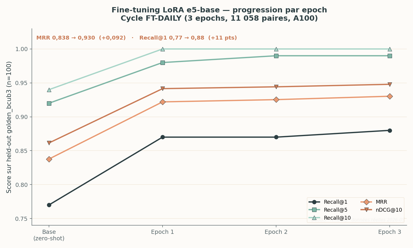Progression of retrieval metrics (Recall@1/@5/@10, MRR, nDCG) over three epochs of LoRA e5-base training, measured on the BCUB3 golden n=100. FT-DAILY cycle of 05/28: e5-base zero-shot (“Base” point) then three LoRA epochs. MRR rises from 0.838 to 0.930.

On the FT-DAILY-2026-05-28 cycle, the base model (e5-base without fine-tune) already starts at MRR 0.838 on the golden, and LoRA fine-tuning carries it to 0.930 in three epochs (+0.092). Recall@10 reaches 1.0 from epoch 1 — and stays there: the golden saturates (more on this in the limits). Recall@1, however, keeps progressing to 0.88, confirming that the gain is not just a ceiling illusion.

Gains vs the production baseline

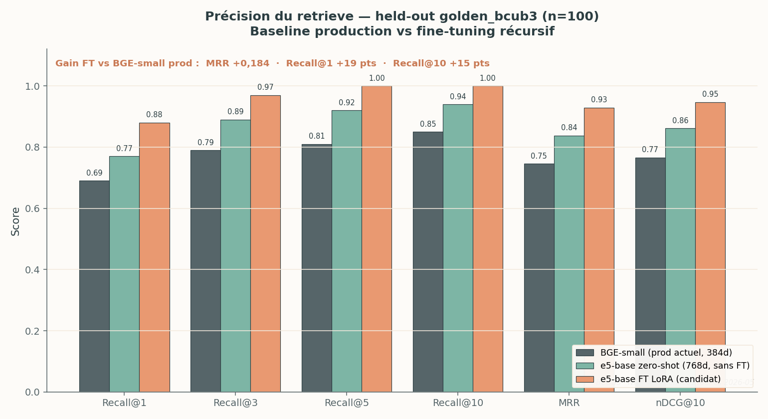Comparison of Recall@1/@3/@5/@10, MRR, nDCG between BGE-small in production, e5-base zero-shot, and fine-tuned e5-base LoRA. Three models on the same golden n=100. The gain decomposes: half comes from the base-model change (BGE → e5), the other half from fine-tuning.

This is the most important figure for judging the value of the operation. Three columns:

BGE-small (the model in production today, 384 dimensions): MRR 0.745 on this golden.
e5-base zero-shot (768 dimensions, without fine-tune): MRR 0.838.
e5-base fine-tuned LoRA (the candidate): MRR 0.929.

The candidate’s total gain over production is +0.184 MRR, +19 points of Recall@1, and +15 points of Recall@10. An honest and instructive detail: more than half the gain comes simply from changing the base model (BGE → e5), before any fine-tune. Fine-tuning adds the specialization layer on top.

A note on baselines. The documented historical threshold in the Nika doctrine is an MRR of 0.674 for BGE-small. The 0.745 value above is what BGE-small obtains on the current BCUB3 golden (n=100), a different set. We cite both for transparency: the real gain is always read at constant test set, column against column.

The recursive loop, cycle by cycle

The header figure shows the essential: across three successive cycles, the candidate’s golden MRR (0.9162 → 0.9231 → 0.9292) progresses but stays below the v1 incumbent (0.9408) and below the gate threshold (0.9358). Real verdicts:

Cycle	Date	Epochs	Pairs	Candidate golden MRR	Verdict	Cost
CONTINUOUS-FT-2	05/25	1	—	0.9162	REJECTED (golden saturated, 1 epoch < mature 3-epoch checkpoint)	$0.115
CONTINUOUS-FT-3	05/26	3	10,144 (+1,325)	0.9231	ROLLBACK (conversational pairs off-distribution from the golden)	$0.313
FT-DAILY	05/28	3	11,058	0.9292	GO golden, but HITL cutover	$0.310
FT-DAILY	05/29	3	+0 new pair	incumbent parity	GO (Δ vs incumbent +0.002)	$0.345

Three concrete takeaways:

The gate does its job. At cycle FT-3, adding 1,325 live conversational pairs lowered the golden MRR (0.9231 < the incumbent 0.9408): those pairs are off-distribution relative to the documentary-retrieval target. The system performed a clean rollback to the incumbent. More data is not always better.
No automatic cutover. Even at the FT-DAILY cycle where the candidate finally beats the incumbent (+0.0008, a decisive but tiny margin), the production promotion stays HITL (human-in-the-loop): the human validates. The active adapter in production remains CONTINUOUS-FT-3.
The cost is negligible — around $0.30 per cycle on an hourly-rented A100. The limiting factor is not compute, it is the evaluation discipline.

The Funes paradox

”Funes the Memorious”

In Borges’s short story, Ireneo Funes, after a fall from a horse, remembers everything: every leaf of every tree he has seen, every instant in its smallest detail. And yet, Borges writes, “to think is to forget differences, to generalize, to abstract.” Funes, unable to forget, is unable to think. His perfect memory is a prison.

At the model level: catastrophic forgetting

The Funes paradox has an exact technical equivalent: catastrophic forgetting. If you specialize a model too violently on a singular corpus — your corpus — it forgets the generalist skills acquired during pre-training. Conversely, a model that wanted to retain everything without abstracting anything would never generalize. Compression and selective forgetting are the condition of intelligence, for an agent as for Funes.

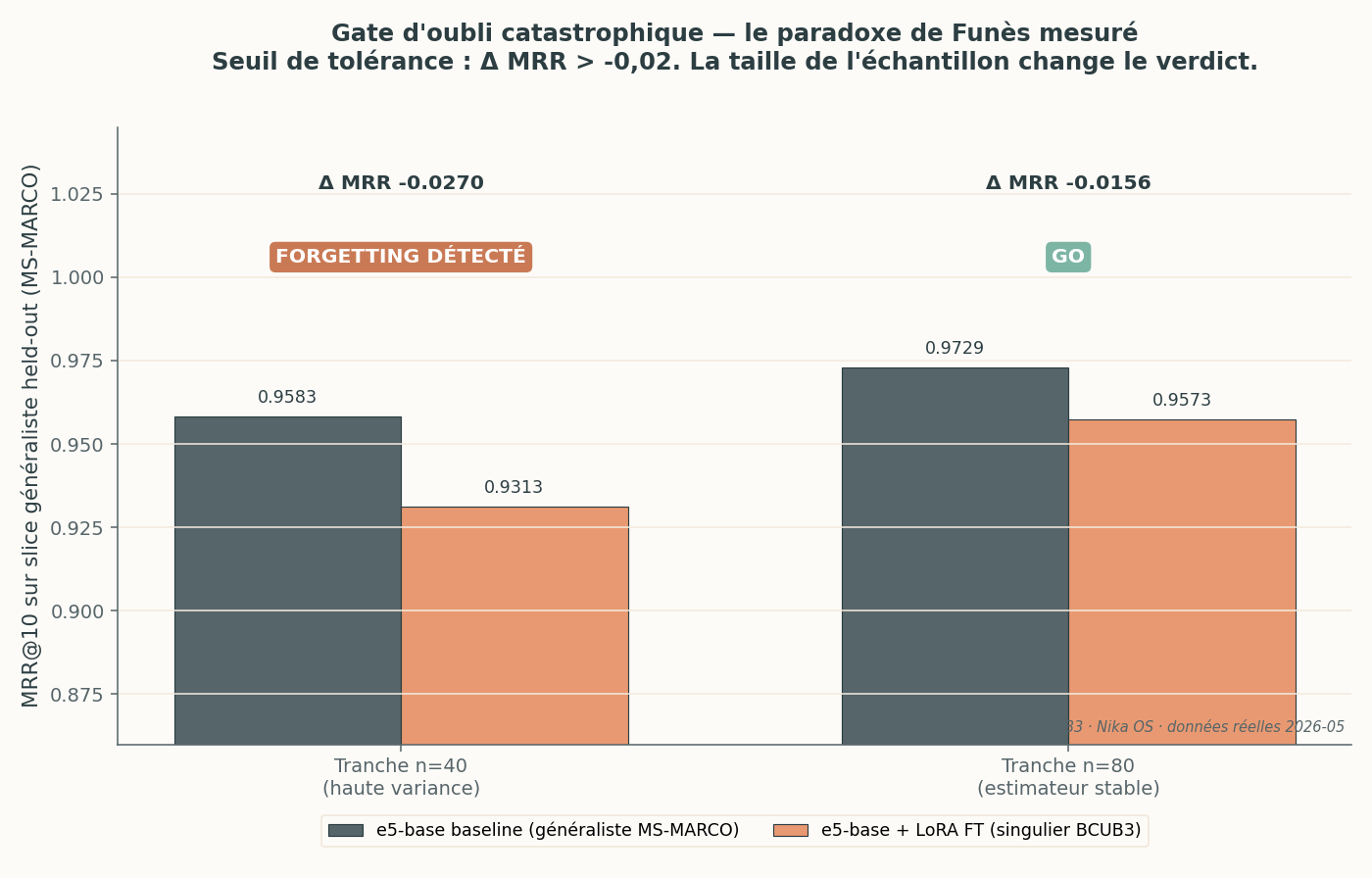Catastrophic-forgetting gate: generalist MRR (MS-MARCO) of the baseline vs fine-tuned model, on a slice of 40 then 80 questions. The verdict flips from FORGETTING DETECTED to GO. The same forgetting measure, on two sample sizes. At n=40, the −0.027 gap exceeds the tolerance threshold (−0.02) and triggers an alarm. At n=80, the gap drops to −0.016: GO. Variance, not forgetting, explained the alarm.

This is where the “effect size vs sample” pedagogy becomes concrete. At the FT-DAILY cycle, the forgetting gate ran twice:

Slice n=40: generalist MRR baseline 0.9583 → fine-tuned 0.9313, i.e. Δ = −0.027. With the tolerance threshold at −0.02, verdict: FORGETTING_DETECTED.
Slice n=80 (rerun, sample doubled): baseline 0.9729 → fine-tuned 0.9573, i.e. Δ = −0.016. Verdict: GO.

The initial alarm came from the variance of a too-small sample, not from genuine forgetting. On 40 questions where Recall@5 and Recall@10 are already 1.0 for both models, MRR is extremely sensitive to a few rank inversions. This is exactly why you do not decide on a tiny n.

The three mandatory safeguards

Recursive fine-tuning is only defensible because it embeds three cumulable protections against Funes:

Rehearsal / replay. At each mini-batch, we re-inject samples from the original generalist corpus (MS-MARCO, MIRACL, BEIR) mixed with the singular BCUB3 data, with a mixing coefficient. The model does not drift toward the recent corpus alone.
Permanent held-out generalist evaluation. In addition to the BCUB3 golden, we keep a generalist slice never seen during training. If its MRR drops by more than 2 points → rollback. This is precisely the gate in the figure above.
Pre-FT checkpoint + automatic rollback. Before each cycle, we save the model’s state. If the evaluation regresses, we revert to the incumbent without debate. The REJECTED and ROLLBACK verdicts in the table above are this mechanism in action.

Without these three safeguards, you reproduce Funes’s error: memorize everything of the present, forget everything of the past.

The honest risk framing

Risk α: “it feels better” without numbers

Risk α (false positive) is acting when you should not have — promoting a model that feels better but is not. The countermeasure is a hard rule: nothing ships on an impression. You need a measured gain, on a held-out test set, above the incumbent.

The canonical example at Nika is documented: an attempt to improve retrieval through a post-hoc score boost (re-weighting results after the fact, inspired by a Kelly-Taguchi-Weibull probabilistic framework) made MRR regress from 0.674 to 0.358 — nearly half. The idea looked attractive on paper; the measurement killed it. Since then, any post-hoc score re-weighting goes through a mandatory empirical gate before integration. What works in production is the opposite: embedding the probabilistic logic inside the model (at the activation level and as tunable hyperparameters), never as a post-hoc score bonus.

The MiniLM lesson: small dataset, counterproductive fine-tune

An earlier experiment (May 18) confirms it by the absurd. A fine-tune of all-MiniLM-L6-v2 on only 50 pairs, 1 epoch, degraded the model: Recall@1 from 0.227 to 0.182 (−0.045), Recall@3 from 0.455 to 0.318 (−0.136). Too little data, and the fine-tune hurts. This justifies the scale of the current cycles (11,000+ pairs, 3 epochs) and the move to GPU.

The limits of this study (stated explicitly)

The golden set saturates. At n=100 with partly synthetic questions, Recall@5 and Recall@10 reach 1.0: only MRR (and Recall@1) remain discriminating. A larger and harder golden, built on real queries, is the next step.
The forgetting slices are small (n=40, n=80). As seen, the verdict flips with size. Stable estimates require a larger slice, which the cron now uses.
The coverage of the re-embedded corpus is partial. During the test migration to the 768d collection, only 619 points out of 355,777 were re-embedded (0.2%) — the rest (emails, invoices, harvested documents) lives in pipelines not replayed for this test. Consequence: on the aggregate all-queries evaluation, Recall@10 drops by −0.02 — not because the model is worse, but because the searched content was not yet re-ingested. On the specifically BCUB3/Nika probes, by contrast, the new model wins 3 cases out of 5, sometimes massively. This is a coverage gap, not a model regression — and distinguishing it honestly is the whole point of a serious risk framework.

FAQ

What is recursive embedding fine-tuning?

It is the periodic, automated retraining of the model that turns text into vectors, on a corpus’s new data, with a strict rule: a new version is promoted to production only if it beats the old one on a held-out test set. Each cycle chains LoRA training, golden evaluation, generalist-forgetting check, then promotion (cutover) or revert (rollback).

What is the difference between Recall@k, MRR, and nDCG?

Recall@k measures whether the right document is returned in the top k results (coverage). MRR rewards ranking it high (1/rank of the first correct result). nDCG refines further by logarithmically penalizing correct answers placed low and accounting for graded relevance. For a RAG, MRR is the most important because the LLM mostly reads the first passages.

What is catastrophic forgetting in fine-tuning?

It is the loss of a model’s generalist skills when you specialize it too much on a singular corpus — the Funes paradox applied to the model: retaining everything of the present makes it forget the past. It is measured by evaluating the fine-tuned model on a generalist slice never seen during training; if its score drops beyond a threshold, promotion is refused.

How do you guard against catastrophic forgetting?

Three cumulable techniques: (1) rehearsal/replay — re-injecting samples from the original generalist corpus during training; (2) a permanent held-out generalist evaluation acting as a safeguard; (3) a pre-training checkpoint with automatic rollback if the evaluation regresses. Keeping the backbone frozen via LoRA is a fourth protection, by construction.

Why is a gain measured on 40 questions not reliable?

Because the variance of a small sample dominates the signal. In a real case measured at Nika, an MRR gap of −0.027 on 40 questions (beyond the alarm threshold) fell to −0.016 — below the threshold — as soon as it moved to 80 questions. Effect size must always be read alongside sample size: a gap on too few cases is not proof.

Does fine-tuning always improve the model?

No. On a too-small dataset (50 pairs, one measured case), the fine-tune degraded Recall@1 by −0.045. And adding off-distribution data (conversational pairs on a documentary-retrieval target) lowered the golden MRR and triggered a rollback. More data or more training are only worth it if evaluated — that is the whole point of the empirical gate.

Going further

This article is part of our technical foundation on RAG and applied AI. The bold terms link to the BCUB3 technical glossary. Related articles:

Methodology: all the curves in this article come from the real training and evaluation logs of the Nika OS recursive fine-tuning loop (cycles CONTINUOUS-FT-2/3 and FT-DAILY, May 25–29, 2026), on NVIDIA A100 GPU. Deterministic seed 42. No curve value has been reconstructed; missing data is flagged as a limitation.