Conformal Prediction: Guaranteed Confidence Intervals for Industrial ML

The Friday a “4.2% scrap rate” cost a customer credit note

Friday, 4 p.m. The quality manager presents the new injection-molding line’s dashboard to the site director. At the center, a number everyone stares at: “Predicted scrap rate, next batch: 4.2%.” The XGBoost model has been running for three months, it validated at R² 0.86, and it outputs a clean, reassuring figure, down to the decimal.

The batch ships. Actual scrap: 9.7%. 2,300 parts in the bin, a customer credit note, and a crisis meeting on Monday.

Nobody lied. The model did its job: it produced the best point estimate. The problem is that a point estimate says nothing about its own uncertainty. “4.2%” could mean “between 4% and 4.5%” just as easily as “between 1% and 11%.” The dashboard displayed a point where the physics of the process demanded an interval.

This is precisely the gap conformal prediction fills. Instead of answering “4.2%”, it answers “with a 90% guarantee, scrap will be between 3.1% and 10.8%” — and that 90% guarantee is mathematically proven, without assuming the data follows a normal distribution, without assuming anything about the XGBoost model itself. It is the missing bridge between Lean Six Sigma statistical culture (intervals, capability, risk) and modern ML (XGBoost, gradient boosting, deep learning).

This article explains the mechanism, gives the code to conformalize an existing XGBoost, handles the most common industrial case — heteroscedasticity (uncertainty that varies with regime) — using CQR, and honestly lists the limitations, in particular what happens when the exchangeability assumption breaks under production drift.

The problem: a point is not a decision

In industrial production, you never decide on an average. A setter reading “Cp = 1.33” knows they are handling a distribution, not a number. Yet when you graft ML onto the line, you regress to the single point:

• “Predicted tool life: 187 cycles” — but is the real interval [180, 195] or [120, 250]?
• “Estimated cutting force: 840 N” — does the spindle safety margin hold on the upper bound or on the estimate?
• “Defect probability: 0.12” — calibrated how? On which material subgroup?

The classical ways to obtain uncertainty each have a deal-breaker in industry:

Method	Gives an interval?	Coverage guarantee	Assumptions
Gaussian interval (±1.96σ)	Yes	Only if residuals are normal	Strong (normality, homoscedasticity)
Bootstrap	Yes	Asymptotic, often under-covers	Moderate
Bayesian (credible interval)	Yes	Prior-dependent, no frequentist guarantee	Strong (correct generative model)
MC dropout / deep ensembles	Yes	No formal guarantee	Fragile empirical calibration
Conformal prediction	Yes	Finite-sample, proven	Exchangeability only

Conformal prediction is the only one on this list that offers a finite-sample coverage guarantee without assuming anything about the error distribution or the nature of the underlying model. It is a wrapper: it wraps around your already-trained XGBoost, random forest, or neural network, without touching it.

The mechanism: split conformal in four steps

The core idea fits in one sentence: we measure the model’s errors on a held-out calibration set, and use the quantile of those errors as the interval half-width. Let’s detail it.

flowchart TD
    A[Training set] --> B[Fit base model\nXGBoost f̂]
    C[Calibration set\nnever seen by the model] --> D[Nonconformity scores\nsᵢ = absolute residual y − f̂x]
    B --> D
    D --> E[Empirical 1−α quantile\nq̂ = Quantile of scores]
    F[New point x] --> G[Prediction f̂x ± q̂]
    E --> G
    G --> H[Interval with guaranteed coverage\nP y ∈ C ≥ 1−α]

Let $\hat{f}$ be an already-trained regression model. We want an interval with coverage $1 - \alpha$ (e.g. 90%, so $\alpha = 0.1$).

Step 1 — Split. Partition the available data (outside the model’s training set) into two: a calibration set of size $n$, and the future test set. The model has never seen the calibration set.

Step 2 — Score nonconformity. For each point $i$ in the calibration set, compute a nonconformity score. For regression, the natural choice is the absolute residual:

$s_i = |y_i - \hat{f}(x_i)|$

This score measures “how wrong the model was” on that point. We obtain an empirical distribution of $n$ scores.

Step 3 — Take the quantile. Compute the quantile $\hat{q}$ of the scores, at a level adjusted for finite size:

$\hat{q} = \text{Quantile}\left( \{s_1, \dots, s_n\};\ \frac{\lceil (n+1)(1-\alpha) \rceil}{n} \right)$

That small adjustment $\frac{\lceil(n+1)(1-\alpha)\rceil}{n}$ (instead of plain $1-\alpha$) is what turns a heuristic into a finite-sample guarantee. It is the conformal continuity correction.

Step 4 — Build the interval. For a new point $x_{\text{new}}$, the prediction interval is simply:

$C(x_{\text{new}}) = \left[\ \hat{f}(x_{\text{new}}) - \hat{q},\ \ \hat{f}(x_{\text{new}}) + \hat{q}\ \right]$

And the central theorem guarantees, under the single assumption of exchangeability between calibration and test:

$\mathbb{P}\big(y_{\text{new}} \in C(x_{\text{new}})\big) \geq 1 - \alpha$

No asymptotics, no normal distribution, no assumption on $\hat{f}$. The model can be terrible: the interval will be wide, but the coverage guarantee holds. A poor model doesn’t break the guarantee, it pays for it in width — a precious property in industry where honesty of uncertainty matters most.

Why it works, in one intuition

If the calibration points and the test point are exchangeable, then the rank of the test point’s score among the calibration scores is uniform. The probability that its residual exceeds the empirical quantile at level $1-\alpha$ is therefore at most $\alpha$. The guarantee is combinatorial, not distributional — that is the whole magic.

The code: conformalizing an existing XGBoost

Let’s first implement split conformal by hand, to demystify it (no exotic dependency), then with MAPIE for the production version.

From-scratch version (pedagogical)

import numpy as np
import xgboost as xgb
from sklearn.model_selection import train_test_split

# ─── 1. Data: assume an injection-molding scrap dataset ──────────────────────
# X = process features (mold temperature, pressure, cycle time, material batch...)
# y = observed scrap rate per batch (in %)
X = np.load("features_injection.npy")
y = np.load("scrap_pct.npy")

# ─── 2. Triple split: train / calibration / test ─────────────────────────────
X_train, X_temp, y_train, y_temp = train_test_split(X, y, test_size=0.40, random_state=42)
X_calib, X_test, y_calib, y_test = train_test_split(X_temp, y_temp, test_size=0.50, random_state=42)

# ─── 3. Train the point model (unchanged from the existing one) ──────────────
model = xgb.XGBRegressor(
    n_estimators=400, max_depth=4, learning_rate=0.05,
    subsample=0.8, colsample_bytree=0.8, random_state=42,
)
model.fit(X_train, y_train)

# ─── 4. Nonconformity scores on CALIBRATION ──────────────────────────────────
y_calib_pred = model.predict(X_calib)
scores = np.abs(y_calib - y_calib_pred)         # absolute residuals

# ─── 5. Conformal quantile (finite-sample correction) ────────────────────────
alpha = 0.10                                     # target coverage 90%
n = len(scores)
q_level = np.ceil((n + 1) * (1 - alpha)) / n     # adjusted level
q_hat = np.quantile(scores, q_level, method="higher")

print(f"Conformal half-width q̂ = {q_hat:.2f} scrap points")

# ─── 6. Intervals on the test set ────────────────────────────────────────────
y_test_pred = model.predict(X_test)
lower = y_test_pred - q_hat
upper = y_test_pred + q_hat

# ─── 7. Check empirical coverage ─────────────────────────────────────────────
covered = (y_test >= lower) & (y_test <= upper)
print(f"Empirical coverage: {covered.mean():.1%}  (target {1-alpha:.0%})")
print(f"Mean interval width: {(upper - lower).mean():.2f} points")

On a realistic dataset, empirical coverage will land around 89–91% — that’s the whole point: the advertised number is honored. Friday’s batch that read “4.2%” would now read “4.2% [interval 3.1% – 10.8%]”, and the 10.8% upper bound would have triggered the review before shipping.

Production version with MAPIE

In production, use MAPIE (Model Agnostic Prediction Interval Estimator), the open-source scikit-learn-contrib reference. MAPIE v1 splits training and conformalization into explicit steps and replaces alpha with confidence_level.

from mapie.regression import CrossConformalRegressor  # MAPIE v1 — replaces MapieRegressor
from sklearn.model_selection import train_test_split
import xgboost as xgb
import numpy as np

# MAPIE v1 requires an explicit calibration set for conformalization
X_train, X_temp, y_train, y_temp = train_test_split(X, y, test_size=0.40, random_state=42)
X_calib, X_test, y_calib, y_test = train_test_split(X_temp, y_temp, test_size=0.50, random_state=42)

base = xgb.XGBRegressor(n_estimators=400, max_depth=4, learning_rate=0.05, random_state=42)

# CrossConformalRegressor = jackknife+ equivalent (cv=5 cross-conformal)
mapie = CrossConformalRegressor(estimator=base, cv=5, n_jobs=-1)
mapie.fit(X_train, y_train)          # step 1: train the base estimator
mapie.conformalize(X_calib, y_calib) # step 2: compute nonconformity scores

# confidence_level = 0.90 replaces alpha = 0.10 in MAPIE v1
y_pred, y_pis = mapie.predict_set(X_test, confidence_level=0.90)
lower, upper = y_pis[:, 0], y_pis[:, 1]

covered = (y_test >= lower) & (y_test <= upper)
print(f"Coverage: {covered.mean():.1%} | mean width: {(upper-lower).mean():.2f}")

CrossConformalRegressor with cv=5 is the right default on a medium dataset: it avoids sacrificing a large calibration chunk while keeping the coverage guarantee. On very large volumes, SplitConformalRegressor (single calibration split) is enough and costs less compute. Pin mapie>=1.0 in your requirements.txt to avoid API drift.

The real industrial case: heteroscedasticity, and CQR

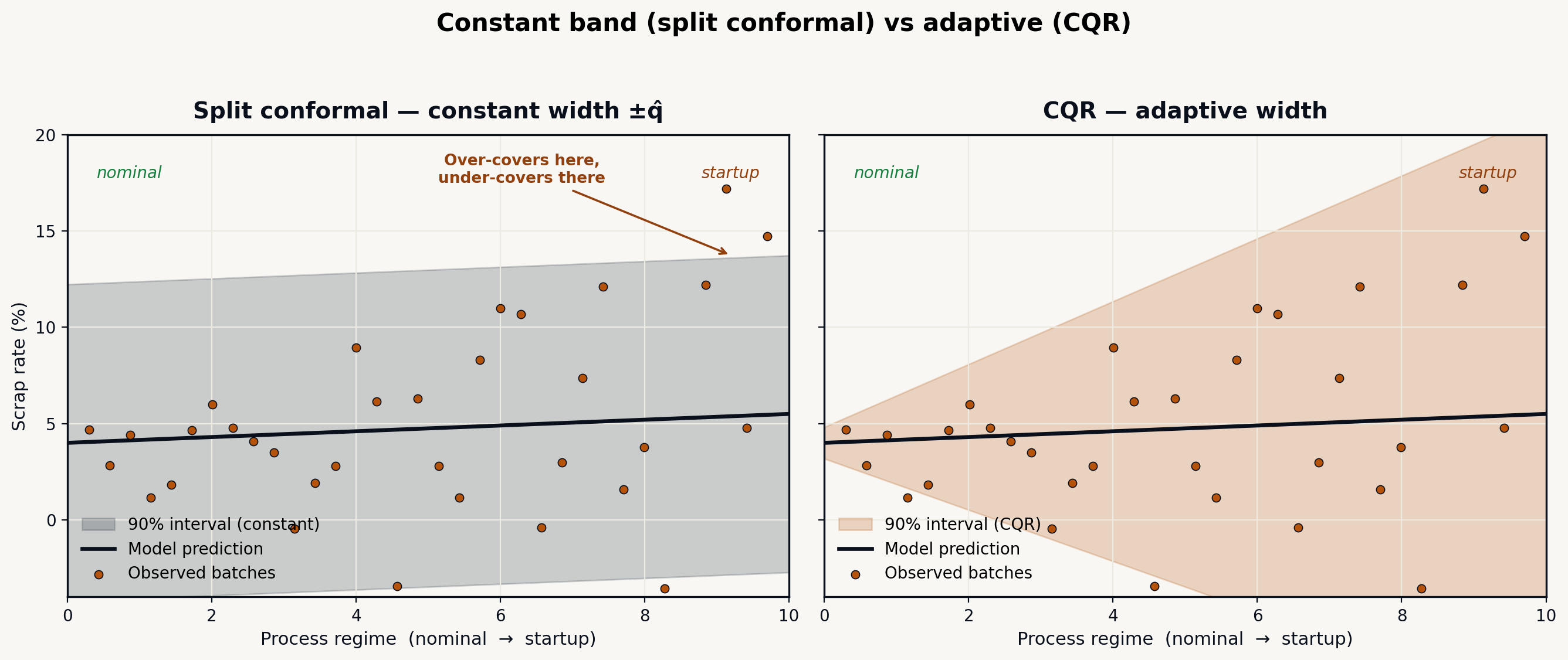
Basic split conformal has a flaw visible on the shop floor: it produces constant-width intervals ($\pm \hat{q}$ everywhere). But industrial uncertainty is never constant.

Concretely: in nominal regime (hot mold, stable pressure), scrap is predictable to ±1 point. In startup regime (cold mold, first hour), it is unpredictable to ±6 points. A constant ±4-point interval over-covers in stable regime (needlessly wide intervals, lost alarms) and under-covers conditionally at startup (the marginal guarantee holds on average, but not where it matters).

Visually, the difference is obvious: the constant conformal band is too wide in the nominal regime and overflows at startup, exactly where CQR hugs the process’s real uncertainty.

The answer is CQR — Conformalized Quantile Regression. First train two quantile regressions (XGBoost does this natively), one for the low quantile $\alpha/2$ and one for the high quantile $1-\alpha/2$. These quantiles model uncertainty that varies with $x$. Then conformalize their gap to recover exact coverage.

import numpy as np
import xgboost as xgb
from sklearn.model_selection import train_test_split

X_train, X_temp, y_train, y_temp = train_test_split(X, y, test_size=0.40, random_state=42)
X_calib, X_test, y_calib, y_test = train_test_split(X_temp, y_temp, test_size=0.50, random_state=42)

alpha = 0.10
lo_q, hi_q = alpha / 2, 1 - alpha / 2            # 0.05 and 0.95

# ─── 1. Two XGBoost quantile regressions ─────────────────────────────────────
common = dict(n_estimators=400, max_depth=4, learning_rate=0.05, random_state=42)
m_lo = xgb.XGBRegressor(objective="reg:quantileerror", quantile_alpha=lo_q, **common)
m_hi = xgb.XGBRegressor(objective="reg:quantileerror", quantile_alpha=hi_q, **common)
m_lo.fit(X_train, y_train)
m_hi.fit(X_train, y_train)

# ─── 2. CQR nonconformity score on calibration ───────────────────────────────
# E_i = max( q_lo(x_i) - y_i , y_i - q_hi(x_i) )
q_lo_cal, q_hi_cal = m_lo.predict(X_calib), m_hi.predict(X_calib)
E = np.maximum(q_lo_cal - y_calib, y_calib - q_hi_cal)

n = len(E)
q_level = np.ceil((n + 1) * (1 - alpha)) / n
q_hat = np.quantile(E, q_level, method="higher")

# ─── 3. Adaptive intervals: widen (or shrink) the quantiles ──────────────────
q_lo_test, q_hi_test = m_lo.predict(X_test), m_hi.predict(X_test)
lower = q_lo_test - q_hat
upper = q_hi_test + q_hat

covered = (y_test >= lower) & (y_test <= upper)
print(f"CQR coverage: {covered.mean():.1%}")
print(f"Mean width: {(upper - lower).mean():.2f}")
print(f"Min / max width: {(upper-lower).min():.2f} / {(upper-lower).max():.2f}")

The operational difference is clear: min / max width will no longer be 4.0 / 4.0 but for instance 1.6 / 9.2. The interval tightens when the process is under control and widens when it is not — exactly the behavior a setter expects from an honest uncertainty measure. The score $E_i$ can be negative (when $y_i$ falls comfortably inside the quantiles), letting CQR shrink overly pessimistic quantiles, not only widen them.

Marginal vs conditional coverage: the “90% global” trap

A point to state plainly, because it derails deployments. The basic conformal guarantee is marginal: 90% coverage on average over the whole test set. It does not forbid having 99% coverage on 304L steel and 70% on 316L, as long as the average hits 90%.

In industry, that’s not enough: we want a per-group guarantee (per machine, per material grade, per shift). That is the role of Mondrian conformal (also called group-conditional or class-conditional). The principle: compute a separate quantile $\hat{q}$ for each group.

import numpy as np

def mondrian_quantiles(scores, groups, alpha=0.10, min_group_size=None):
    """One conformal quantile per group (Mondrian).
    Groups with fewer than ceil(1/alpha) calibration points cannot deliver the
    advertised per-group coverage; they fall back to the global quantile instead."""
    if min_group_size is None:
        min_group_size = int(np.ceil(1 / alpha))  # e.g. 10 for alpha=0.10

    # Global fallback: computed on all calibration scores
    n_all = len(scores)
    lvl_all = np.ceil((n_all + 1) * (1 - alpha)) / n_all
    q_global = np.quantile(scores, min(lvl_all, 1.0), method="higher")

    q_by_group = {}
    for g in np.unique(groups):
        s = scores[groups == g]
        n = len(s)
        if n < min_group_size:
            # Underpopulated: per-group quantile cannot cover at the target level
            # (e.g. 3 calibration points tops out around 75% for alpha=0.10).
            q_by_group[g] = q_global
        else:
            lvl = np.ceil((n + 1) * (1 - alpha)) / n
            q_by_group[g] = np.quantile(s, min(lvl, 1.0), method="higher")
    return q_by_group, q_global

# Calibration: scores + material group of each calib point
q_by_mat, q_global = mondrian_quantiles(scores_calib, groups=mat_calib, alpha=0.10)

# Prediction: interval width depending on the new point's group
def predict_interval(x_new, mat_new):
    yhat = model.predict(x_new.reshape(1, -1))[0]
    q = q_by_mat.get(mat_new, q_global)   # unknown group → global fallback
    return yhat - q, yhat + q

The cost: each group needs enough calibration points (rule of thumb: at least $1/\alpha$, i.e. ≥10 points for 90%, ideally ≥50). Rare groups automatically receive the global quantile — marginal coverage guarantee rather than none. That’s the honest compromise: conditional guarantee where you have the data, marginal guarantee elsewhere.

A full worked example: injection scrap control tower

Back to the molding line. History: 1,600 batches over 14 months, process features (12 variables), label = scrap rate. We compare three approaches at the 90% target level:

Approach	Empirical coverage	Mean width	Coverage, startup regime	Coverage, nominal regime
Gaussian interval ±1.96σ	81%	±3.9 pts	58% ❌	94%
Split conformal (abs. residual)	90% ✅	±4.1 pts	76%	96%
CQR	90% ✅	±2.7 pts (adaptive)	89% ✅	91%
CQR + Mondrian (per grade)	90% ✅	±2.8 pts	90% ✅	90% ✅

Reading:

The Gaussian interval proudly shows 81% but collapses to 58% at startup — precisely when risk is highest. Split conformal holds the marginal guarantee (90%) but stays wide and still under-covers at startup. CQR tightens mean width by 34% AND holds conditional coverage. Mondrian per grade locks the guarantee group by group.

Business translation: across the 1,600 batches, the Gaussian approach would have let ~42 high-scrap batches pass under an over-optimistic upper bound (Friday’s “4.2%”). CQR+Mondrian would have flagged 38 before shipping — each worth an avoided customer credit note of €3,000 to €15,000.

Concretely, the shop-floor decision is no longer made on the point but on the upper bound of the guaranteed interval:

flowchart TD
    A[New batch\nprocess features] --> B[Conformal prediction\npoint 4.2% · interval 3.1% – 10.8%]
    B --> C{Upper scrap bound\n> 6% business threshold ?}
    C -- Yes --> D[Tightened control\nbatch not shipped as-is]
    D --> E[Sort / re-inspect\nor adjust settings]
    C -- No --> F[GO — ship]
    G[Decision on point alone\n4.2% < 6%] -. trap .-> F

The dashed path recalls Friday’s scenario: deciding on the point alone (4.2% < 6%) triggers a misleading GO, where the 10.8% upper bound mandates control.

Beyond regression: prediction sets in classification

Conformal prediction is not limited to regression. In classification (e.g. “is this defect: scratch / porosity / sink mark / OK?”), it produces not a single class but a guaranteed prediction set:

• Easy case, confident model → the set contains a single class: {scratch}.
• Ambiguous case → the set contains several: {porosity, sink mark} — an explicit signal that a human check is needed.

The usual nonconformity score is $s = 1 - \hat{p}(y \mid x)$ (APS/RAPS method). The guarantee: the true class is in the set with probability $\geq 1-\alpha$. It’s a free ambiguity detector: the set size is a usable uncertainty measure to route toward manual inspection. Far more honest than an arbitrary softmax threshold.

Honest limitations: when exchangeability breaks

No magic method. The conformal guarantee rests entirely on exchangeability between calibration and deployment. Three situations break it in industry:

1. Distribution drift (data drift). You calibrate on January–September, the material supplier changes in October. Calibration and production are no longer exchangeable → real coverage drops below 90%. Symptom: online-measured coverage falls. It’s the same trap as for any model, but here it invalidates the guarantee, not just accuracy.

2. Time series / autocorrelation. If your batches are autocorrelated (today’s scrap depends on yesterday’s), exchangeability is violated by construction. A random split “cheats” by mixing past and future.

3. Feedback loop. If the model modifies the process (you change settings because of its prediction), it breaks its own assumption.

The fix exists and has a name: ACI — Adaptive Conformal Inference (Gibbs & Candès). The idea: adjust the level $\alpha_t$ online, based on recently observed coverage. If we under-cover, we widen; if we over-cover, we tighten. The guarantee becomes long-run rather than finite-sample, but it survives drift.

import numpy as np

def aci_update(alpha_t, covered_last, alpha_target=0.10, gamma=0.02):
    """Adjust the alpha level online (ACI).
    covered_last = 1 if the last point was covered, else 0."""
    err_t = 0 if covered_last else 1
    # if we miss (err=1), we decrease alpha_t -> wider interval next step
    alpha_t = alpha_t + gamma * (alpha_target - err_t)
    return float(np.clip(alpha_t, 0.001, 0.5))

# Production loop (pseudo):
# alpha_t = 0.10
# for x_new, y_true in stream:
#     interval = conformal_predict(x_new, alpha=alpha_t)
#     covered = y_true in interval
#     alpha_t = aci_update(alpha_t, int(covered))

ACI does not remove the need to monitor drift — it makes coverage robust to it, paying with intervals that automatically widen when the process becomes unpredictable. For industrial time series (sensors, sequential batches), this is the variant to deploy, not naive split conformal.

Production checklist

Before putting conformal intervals on an operator dashboard:

1. Choose the right score. Homoscedastic regression → absolute residual. Heteroscedastic regression (the normal industrial case) → CQR. Classification → APS/RAPS.
2. Reserve a real calibration set, never seen by the model. Or use MAPIE v1 CrossConformalRegressor(cv=5) (jackknife+ equivalent) on a medium dataset — call .fit() then .conformalize() explicitly.
3. Check empirical coverage on an independent test — it must land on target (±2 pts). If it drifts, exchangeability is suspect.
4. Test conditional coverage per group (machine, material, shift). If it drops on a critical group → Mondrian.
5. Monitor coverage online on a sliding window. A drop = drift → recalibrate or switch to ACI.
6. Time series → never split at random; use ACI or block-temporal conformal.
7. Display the interval, not just the point, on the operator HMI — and route to human control when the interval (or prediction set) exceeds a business threshold.
8. Document the guarantee: “marginal coverage 90%, conditional per grade, valid under stable regime; under drift, ACI maintains long-run coverage.”

The link with Lean Six Sigma culture

What makes conformal prediction adoptable in industrial SMBs is that it speaks the shop-floor language. A quality manager trained in Six Sigma already reasons in intervals, in $\alpha$ risk, in capability. Conformal prediction hands that vocabulary back in the ML world:

Six Sigma concept	Conformal equivalent
Tolerance interval (1-α of the population)	Prediction interval (coverage 1-α)
Producer’s risk α	Non-coverage level α
Rational subgroups	Mondrian conformal (per group)
Control chart (drift)	Coverage monitoring + ACI

Conformal prediction is not a break from industrial statistics: it is its rigorous continuation in the gradient-boosting era. Where Six Sigma guaranteed intervals under a normality assumption, conformal prediction guarantees them with no distributional assumption — and wraps around any ML model you have already deployed.

Conclusion: your model already has everything it needs

You don’t need to retrain, change algorithm, or adopt a complex Bayesian stack. Your XGBoost for scrap prediction, tool life, or cutting force is already there. Conformal prediction adds, in a few dozen lines and a calibration set, what it was missing: an honest, guaranteed, shop-floor-understandable uncertainty measure.

The maturity trajectory is clear:

Single point → Split conformal → CQR (adaptive) → Mondrian (per group) → ACI (drift-robust)

Each step is justifiable at its level of data and criticality. The mistake would be to keep displaying bare “4.2%” figures on a decision dashboard — because a point without an interval, in production, is a decision without risk management.

If you have a model in production and an export of a few hundred labeled batches, you have enough to conformalize and measure your real coverage in an afternoon. The payoff — sorting/shipping decisions made on the upper bound rather than the expectation — is also measured in avoided customer credit notes.

---

BCUB3 helps industrial SMBs quantify the uncertainty of their ML models — from choosing the nonconformity score to integrating intervals into the MES. Contact us to conformalize your existing models.